Pytorch Analysis Week 7
Date: 2020/4/4-2020/4/10
Last week, we implemented the PCNN model and learnt what is embedding layer & how to initialize the network with pretrained word2vec.
This week, we are not going to implement new model by ourselves, instead, we will learn how Graph Nerual Network is built using pytorch and analysis the implement of Resnet in torchvision.models folder through the source code proposed in the paper Multi-Label Image Recognition with Graph Convolutional Networks, CVPR 2019.
So today’s topics are as follows:
- Analysis the provided model to learn how to build the model.
- Analysis the basic implement of Resnet which is a built-in model provided in Pytorch framework.
- Question & Summary
Multi-Label Image Recognition with GCN
Introduction
Descriptions about the model:
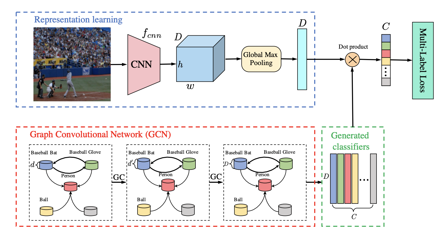
Showed in the above part of image, pretrained ResNet101 was used to capture the image feature([batch_size, 3, W, H] -> [batch_size, D, W, H]), then the Global Max Pooling Layer retrieve the max value of each channel of the output([batch_size, D, W, H] ->[batch_size, D, 1])
Showed in the below part, GCN is used on the graph (nodes are labels, global co-occurrence were used to build edges) to model the inter dependencies between labels. (Inputs are word embedding of the label [C, d] -> [C, D], where, C: number of different labels).
Descriptions about the source code structure: The model were tested on both voc2007 & coco2014(20G) dataset. All Preparations on each datasets are done in coco.py & voc.py separately. util.py provides basic tools such as a converter transforming RGB images into tensor data, AveragePrecisionMeter class to add up the average acc & loss dynamically, and methods for generate the graph we will used in GCN part. model.py, engine.py files provides shared model and train engines which will be used in demo_coco_gcn.py and demo_voc2007_gcn.py to examine the model.
Learn from their code
Module Part
Graph Convolutional Network Recap:
the goal of GCN is to learn a function f(·, ·) on a graph G, which takes feature descriptions and the corresponding correlation matrix as inputs (where n denotes the number of nodes and d indicates the dimensionality of node features), and updates the node features as . Every GCN layer can be written as a non-linear function by
where : is a transformation matrix to be learned, and is the normalized version of correlation matrix A, and h(·) denotes a non-linear operation (LeakyReLU ).
Implement of GCN submodule :
Though Graph Neural Network has been commonly used in most machine learning scope since it first proposed in 2016, unfortunately, there is little support for it in traditional deeplearning framework. So We had to build it from scratch, thankfully it’s powerful but simple model.
class GraphConvolution(nn.Module):
    """
    Simple GCN layer, similar to https://arxiv.org/abs/1609.02907
    """
    def __init__(self, in_features, out_features, bias=False):
        super(GraphConvolution, self).__init__()
        self.in_features = in_features
        self.out_features = out_features
        #  We had to define the parammeter on our own, according to recapation,
        # the parameter of the model is a (in_features, out_feature) Matrix.& bias.
        self.weight = Parameter(torch.Tensor(in_features, out_features))
        if bias:
            self.bias = Parameter(torch.Tensor(1, 1, out_features))
        else:
            self.register_parameter('bias', None)
        self.reset_parameters()

    def reset_parameters(self):
        # initialization of module parameters.
        stdv = 1. / math.sqrt(self.weight.size(1))
        self.weight.data.uniform_(-stdv, stdv)
        if self.bias is not None:
            self.bias.data.uniform_(-stdv, stdv)

    def forward(self, input, adj):
        # implement by only matrix dot product ! what a simple module.
        support = torch.matmul(input, self.weight)
        output = torch.matmul(adj, support)
        if self.bias is not None:
            return output + self.bias
        else:
            return output

    def __repr__(self):
        return self.__class__.__name__ + ' (' \
               + str(self.in_features) + ' -> ' \
               + str(self.out_features) + ')'
complete module :
There are still many thing we can learn from the model shown here. (we mark them within the code.)
class GCNResnet(nn.Module):
    def __init__(self, model, num_classes, in_channel=300, t=0, adj_file=None):
        super(GCNResnet, self).__init__()
        # One : Learning how to make use of part of ResNet in our model.
        # Using. nn.Sequential & the corresponding layer name.
        self.features = nn.Sequential(
            model.conv1,
            model.bn1,
            model.relu,
            model.maxpool,
            model.layer1,
            model.layer2,
            model.layer3,
            model.layer4,
        )
        self.num_classes = num_classes
        self.pooling = nn.MaxPool2d(14, 14)

        self.gc1 = GraphConvolution(in_channel, 1024)
        self.gc2 = GraphConvolution(1024, 2048)
        self.relu = nn.LeakyReLU(0.2)

        _adj = gen_A(num_classes, t, adj_file)
        self.A = Parameter(torch.from_numpy(_adj).float())
        # image normalization
        self.image_normalization_mean = [0.485, 0.456, 0.406]
        self.image_normalization_std = [0.229, 0.224, 0.225]

    def forward(self, feature, inp):
        feature = self.features(feature)
        feature = self.pooling(feature)
        feature = feature.view(feature.size(0), -1)

        inp = inp[0]
        adj = gen_adj(self.A).detach()
        x = self.gc1(inp, adj)
        x = self.relu(x)
        x = self.gc2(x, adj)

        x = x.transpose(0, 1)
        x = torch.matmul(feature, x)
        return x
    # Two : One way to give the pretrain module smaller learning rate.
    #  # define optimizer
    #   optimizer = torch.optim.SGD(model.get_config_optim(args.lr, args.lrp),
    #                     lr=args.lr, momentum=args.momentum,
    #                     weight_decay=args.weight_decay)
    def get_config_optim(self, lr, lrp):
        return [
                {'params': self.features.parameters(), 'lr': lr * lrp},
                {'params': self.gc1.parameters(), 'lr': lr},
                {'params': self.gc2.parameters(), 'lr': lr},
                ]

# the final api to get access to model.
def gcn_resnet101(num_classes, t, pretrained=True, adj_file=None, in_channel=300):
    model = models.resnet101(pretrained=pretrained)
    return GCNResnet(model, num_classes, t=t, adj_file=adj_file, in_channel=in_channel)
What’s the original adj-matrix like ?
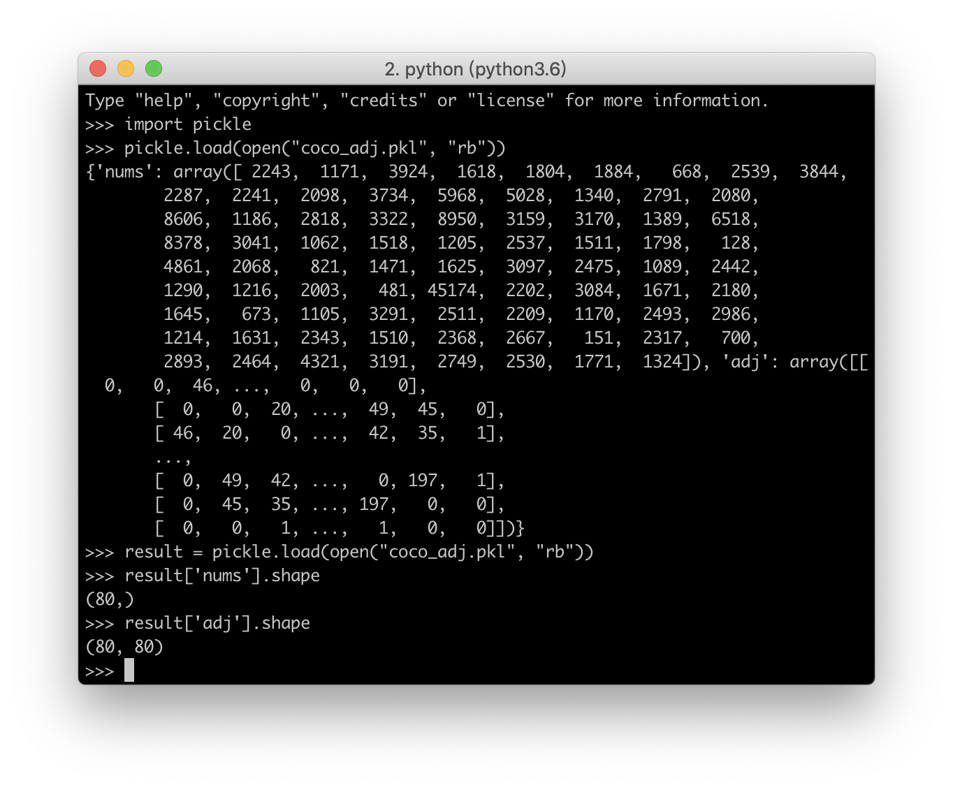
The author has directly provide the original matrix for us, from the statistic below, it contains ‘nums’: counter of how many times each classes(80 in total) occur. ‘adj’: the co-occurrence matrix of the class (80x80).
With help of this code, we can get better sence about the gen_A function provide in util.py
def gen_A(num_classes, t, adj_file):
    import pickle
    result = pickle.load(open(adj_file, 'rb'))
    _adj = result['adj']
    _nums = result['nums']
    # first get the conditional probability _nums[i,j] = P(xj | xi).
    _nums = _nums[:, np.newaxis]
    _adj = _adj / _nums
    # clip with threshold.
    _adj[_adj < t] = 0
    _adj[_adj >= t] = 1
    # normalization processing.
    _adj = _adj * 0.25 / (_adj.sum(0, keepdims=True) + 1e-6)
    # set diag items to 1.
    _adj = _adj + np.identity(num_classes, np.int)
    return _adj

def gen_adj(A):
    # Receive the output of gen_A as input.
    D = torch.pow(A.sum(1).float(), -0.5)
    D = torch.diag(D)
    adj = torch.matmul(torch.matmul(A, D).t(), D)
    return adj
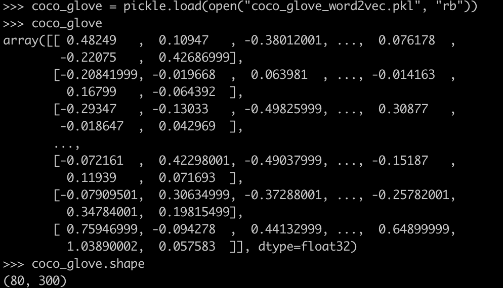
What ‘s the original label embedding format like?
The same as the adj-matrix of coco dataset, the author directly provide the word embedding for the 80 class in coco dataset.
Now we find that one half of the model is built based on the built-in ResNet module. To fathom the model, we should take a look at how the ResNet works.
ResNet Implement in torchvision.models
- In the source code, they first build the conv3x3 & conv1x1 method, which wrap the basic layer nn.Conv2d.
def conv3x3(in_planes, out_planes, stride=1, groups=1, dilation=1):
    """3x3 convolution with padding"""
    return nn.Conv2d(in_planes, out_planes, kernel_size=3, stride=stride,
                     padding=dilation, groups=groups, bias=False, dilation=dilation)


def conv1x1(in_planes, out_planes, stride=1):
    """1x1 convolution"""
    return nn.Conv2d(in_planes, out_planes, kernel_size=1, stride=stride, bias=False)
Cuz the Resnet itself contains various subclass(from resnet18 to resnet152). The large span of the depth of Resnet leads to different network structures. So BasicBlock is used when the depth is lower than 50, while Bottleneck is used when the depth is larger. For connivence, we only show the Bottleneck structure here.
class Bottleneck(nn.Module):
    expansion = 4
    __constants__ = ['downsample']

    def __init__(self, inplanes, planes, stride=1, downsample=None, groups=1,
                 base_width=64, dilation=1, norm_layer=None):
        super(Bottleneck, self).__init__()
        if norm_layer is None:
            norm_layer = nn.BatchNorm2d
        width = int(planes * (base_width / 64.)) * groups
        # Both self.conv2 and self.downsample layers downsample the input when stride != 1
        # Here, with the help of conv1x1 layer we can reduce the "size" of our model
        # which is needed in larger model.
        # Each of conv layer is followed by a batch normalization layer to control the
        # gradient flow. And provide more choice of the model.
        self.conv1 = conv1x1(inplanes, width)
        self.bn1 = norm_layer(width)
        self.conv2 = conv3x3(width, width, stride, groups, dilation)
        self.bn2 = norm_layer(width)
        self.conv3 = conv1x1(width, planes * self.expansion)
        self.bn3 = norm_layer(planes * self.expansion)
        self.relu = nn.ReLU(inplace=True)
        self.downsample = downsample
        self.stride = stride

    def forward(self, x):
        identity = x

        out = self.conv1(x)
        out = self.bn1(out)
        out = self.relu(out)

        out = self.conv2(out)
        out = self.bn2(out)
        out = self.relu(out)

        out = self.conv3(out)
        out = self.bn3(out)

        if self.downsample is not None:
            identity = self.downsample(x)
        # Here is the core of resnet, by adding the identity of input,
        # the model has better ability of makeing subtle changes which is needed
        # to prevent degrading problem.
        out += identity
        out = self.relu(out)

        return out
Now, came to the ResNet class, we only show some core code here to simplify our report.
class ResNet(nn.Module):

    def __init__(self, block, layers, num_classes=1000, zero_init_residual=False,
                 groups=1, width_per_group=64, replace_stride_with_dilation=None,
                 norm_layer=None):
        super(ResNet, self).__init__()
        if norm_layer is None:
            norm_layer = nn.BatchNorm2d
        self._norm_layer = norm_layer

        self.inplanes = 64

          # dilated convolution (Convolution with holes) part, (commonly used in separation.)
        # ...

        self.groups = groups
        self.base_width = width_per_group
        self.conv1 = nn.Conv2d(3, self.inplanes, kernel_size=7, stride=2, padding=3,
                               bias=False)
        self.bn1 = norm_layer(self.inplanes)
        self.relu = nn.ReLU(inplace=True)
        self.maxpool = nn.MaxPool2d(kernel_size=3, stride=2, padding=1)
        self.layer1 = self._make_layer(block, 64, layers[0])
        self.layer2 = self._make_layer(block, 128, layers[1], stride=2,
                                       dilate=replace_stride_with_dilation[0])
        self.layer3 = self._make_layer(block, 256, layers[2], stride=2,
                                       dilate=replace_stride_with_dilation[1])
        self.layer4 = self._make_layer(block, 512, layers[3], stride=2,
                                       dilate=replace_stride_with_dilation[2])

        # using nn.AdaptiveAvgPool2d we can convert out[batch_size, channels, W, H]
        # into any shape [batch_size, channels, x, y]
        # This layer is still used in faster-rcnn, a famous model in detection field.

        self.avgpool = nn.AdaptiveAvgPool2d((1, 1))
        # the last layer is fully connected layer. commonly subplanted.
        self.fc = nn.Linear(512 * block.expansion, num_classes)

           # initialization
        #   ...

    def _make_layer(self, block, planes, blocks, stride=1, dilate=False):
        norm_layer = self._norm_layer
        downsample = None
        previous_dilation = self.dilation
        if dilate:
            self.dilation *= stride
            stride = 1
        if stride != 1 or self.inplanes != planes * block.expansion:
            downsample = nn.Sequential(
                conv1x1(self.inplanes, planes * block.expansion, stride),
                norm_layer(planes * block.expansion),
            )

        layers = []
        layers.append(block(self.inplanes, planes, stride, downsample, self.groups,
                            self.base_width, previous_dilation, norm_layer))
        self.inplanes = planes * block.expansion
        for _ in range(1, blocks):
            layers.append(block(self.inplanes, planes, groups=self.groups,
                                base_width=self.base_width, dilation=self.dilation,
                                norm_layer=norm_layer))

        return nn.Sequential(*layers)

    def _forward_impl(self, x):
        # ...
       def forward(self, x):
        # ...
Summary
- This week, we first learnt how to build GCN on a fixed network, & how gcn works.
- Secondly, we skimmed the implementation of Resnet .
- Next week, we will keep going and have a generalized look on other stoa model and the implementation of them.